Particle Filter for Localization
Particle Filter for Localization
- Note: I wrote this article during grad school and have not revised it since. This is written for simplicity and intuition but not accuracy
In this post I explain how to use particle filters for localization with almost no equations. I have written code which could be used for any robot — you can find the implementation on gitHub.
Localization — the problem
Localization is the ability of a robot to locate itself in the world. For humans, that means knowing where you are (for example: “I’m at the library, next to the main desk” or “I’m at the café having dinner”). Humans usually express location relative to landmarks rather than by giving exact latitude/longitude.
Robots can use sensors (GPS, odometry, range sensors) to estimate position, but sensors have noise and failure modes:
- A GPS in good conditions may give ~2 m accuracy — that’s often too coarse for a robot that has to stay in a lane or follow a narrow path.
- GPS can fail (e.g., inside tunnels), so we need alternative methods.
For outdoor scenarios with many sensors, Kalman filters (and variants) are often used to fuse sensor data into a single estimate. For many indoor robots (where GPS is unavailable or unreliable), particle filters are a practical choice for localization.

Frames
The coordinate frame defines how locations are expressed. For GPS, the origin is latitude=0, longitude=0; for an indoor robot you’ll typically use a custom world frame (for example: place the room origin at (0,0,0)). In a known map the robot and any landmarks are expressed in that world frame, and the robot estimates its pose relative to it.
Particle Filter — intuition
A particle filter estimates the robot’s pose by maintaining many particles (hypotheses). Each particle is a candidate pose; the filter uses sensor measurements (distances to landmarks, etc.) to weigh and resample particles until they concentrate around the true pose.
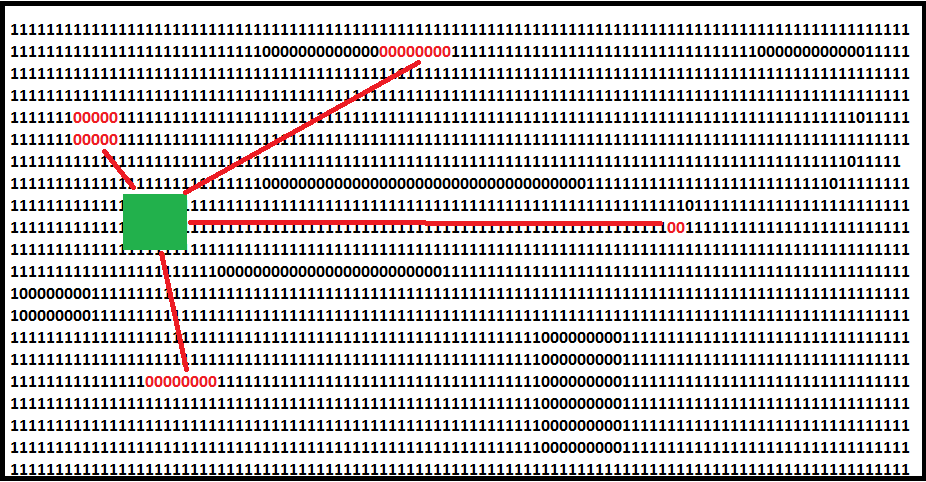
Important constraint: particle filters assume a known map (positions of obstacles and landmarks are known). A simple map representation could be a grid where 1 indicates free space and 0 indicates obstacles; some 0 cells represent landmarks.
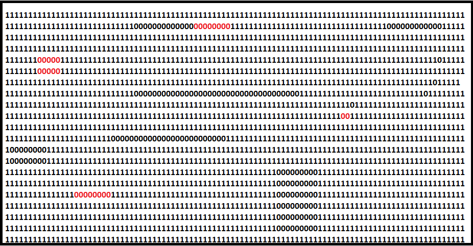
In the figure below the green square is the robot and the red lines indicate range sensor beams to landmarks. The robot localizes by comparing its measured distances to landmarks with the distances a particle would observe if the robot were actually at that particle’s pose.
The algorithm (high level)
- Create
Nparticles. - Move each of the
Nparticles according to the same control input the robot received (e.g., motors commanded to move forward by X). - Measure the robot’s distances to landmarks (from sensors).
- For each particle, compute the distances to those landmarks (from the particle’s pose on the known map).
- Assign a weight to each particle based on how closely that particle’s landmark distances match the robot’s measured distances.
- Normalize the weights so they sum to 1.
- Resample the particle set (with replacement) using the normalized weights — particles with higher weight are more likely to be duplicated.
- Repeat from step 2 (loop continuously).
Step 1 — choose N (number of particles)
Choose N by trial and error relative to map scale and desired accuracy. For example, on a 1000×1000 cm map you might test 2,000 vs 10,000 particles:
- 2,000 particles → ~4 cm accuracy (example)
- 10,000 particles → ~3.8 cm accuracy (example)
Often you see diminishing returns beyond a threshold: increasing from 10,000 to 20,000 particles might yield only tiny improvement but much more computation. Tune N to trade off accuracy vs CPU.
Step 2 — motion (propagate particles)
At each control step, propagate every particle by the same commanded motion the robot received. For example, if the robot moved forward 15 cm north, advance all particles by the same translation (plus optional motion noise to reflect uncertainty). If there was no motion command, skip the motion update and continue with measurement weighting/resampling.
Step 3 — robot measurements to landmarks
At each timestep, the robot measures distances to landmarks using sensors (stereo vision, lidar, ultrasonic, etc.). If your robot lacks range-bearing sensors, this particular algorithm is not suitable.
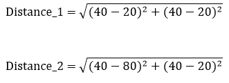
Step 4 — particle measurements to landmarks
For a particle with known coordinates (e.g., (40,40)), and known landmark coordinates (e.g., (20,20) and (80,20)), compute Euclidean distances:
Step 5 — weight particles using sensor uncertainty (Gaussian)
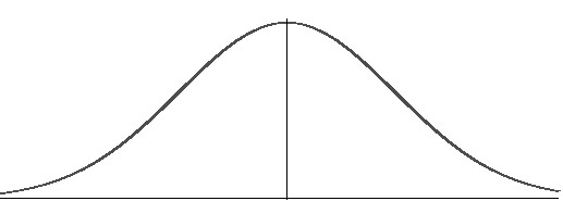
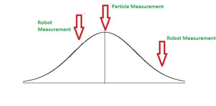
Sensor readings have noise. We model the likelihood of a particle’s predicted distance versus the robot’s measured distance using a probability distribution — typically a Gaussian (normal) distribution. The idea:
- If a particle’s predicted measurement is near the robot’s measured value → high likelihood (high weight).
- If it’s far → low likelihood (low weight).
A uniform distribution would give every value equal probability (not useful here); the Gaussian places higher probability near the mean and lower in the tails.
If you have m landmarks, each particle yields m likelihood values (one per landmark). Multiply those m likelihoods to get the particle’s combined weight (equivalent to the product of independent likelihoods). The result is a single scalar weight per particle. Then normalize across all particles (next step).
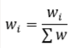
Step 6 — normalize weights
Normalize weights so they sum to 1:
Step 7 — resampling
Resampling is crucial. Think of a bag with N colored balls; drawing N times with replacement gives some repetition and some colors may not be drawn. In particle filters, we draw N particles with replacement, but we bias the draw by particle weights:
- Particles with higher normalized weight are more likely to be drawn multiple times.
- Particles with low weight may disappear from the new set.
After resampling you still have N particles, but the population is concentrated around high-likelihood regions. There are many resampling algorithms (multinomial resampling, systematic resampling, stratified resampling, residual resampling); the basic idea is identical across them — prefer high-weight particles.
Step 8 — repeat
Loop back to Step 2: after resampling, propagate the new particle set with the next control command, measure, reweight, resample, and so on. Over repeated iterations the particle cloud typically converges:
- If many particles converge to a similar pose, take their average as the pose estimate.
- If the particle set collapses to identical particles, that pose is the best estimate (but beware of particle impoverishment; injecting noise or using better resampling methods helps).
Implementation & code
My complete implementation is available on GitHub. The code is written to be generic so it can be adapted to different robots and sensor suites.
Closing notes
Particle filters are conceptually simple and powerful for indoor/landmark-based localization with known maps. The main design choices are:
- number of particles
N(trade accuracy vs compute), - motion and sensor noise models (how you perturb particles and model measurement noise),
- resampling algorithm (to reduce variance and avoid particle depletion),
- representation of the map and landmarks.